DIY xkcd Password Generator

One of the things I'm thankful for today is xkcd. Specifically, I want to talk about the world-famous password strip, which points out that using a few selections from a big list of things (a dictionary) is more random, and yet easier to remember, than a lot of selections from a limited list of things (the keys on your keyboard).

There are even sites which generate xkcd-style passwords for you. Many sites, in fact.

The other day I was using one of these generators to make a password for work. The only problem was that the system that I was logging on to required my password to be between 8 and 16 letters, which is difficult to do when you're dealing with a list of random dictionary words. It also checks to see if you had a string of four or more letters that matched a dictionary word.

To fix this, I needed to have a list of, say, three letter words. Where to find them? Sergey and Larry's search engine helped. For example, here's a list of allegedly legal Scrabble words. Given that, all we need is a script to generate a list of words.

That script is below. What I didn't do was include the words. For one thing I'm not sure about the copyright status of that list. For another, you might want to use your own list. For a third, it would make this post really, really long. So add your own list of words, one per line, between the two EOF lines in the script.

While I was at it, I decided to add a few improvements, towit:

• You can specify the number of words. If you call the script xkcdpass, then
  

  xkcdpass 5
  

  will generate a password using five words from the list. The default is 4, which you can easily change.
• Given the number of words in the list, call it N, and the number of words in the password, call it M, you can generate N^M unique passwords (since strings like thethethethe are perfectly valid). That's a measure of password security, so the script tells you that.
• You have three choices of randomness. In order of security, they are: The bash variable $RANDOM, which can be seeded to the current time, and the linux scripts /dev/urandom and /dev/random. Uncomment the one you like, depending on your level of paranoia.
• It should work on any system that runs bash, including Macs.
• And, of course, I tried to document where I got everything.

So here's the script. Add a comment if you see a problem, or if you just like (or hate) it.

#! /bin/bash

# Generates an xkcd-like password from a list of three-letter words

# Usage

# xkcdpass n

# where n>0 is the number of words in the string.  The default value of
#  n is 4.

# Set the default if needed

if (( $# < 1 ))
then
    nwords=4
else
    nwords=$1
fi

# Set up an array and populate it.
declare -a array
let index=0

# There is a list of acceptable three-letter Scrabble words at
# http://www.yak.net/kablooey/scrabble/3letterwords.html
# Add additional words, if you like, or use a different list.

while read line
do
	array[$index]=$line
	let index=$index+1

# Insert your words between the two EOFs, one per line
# There is a list of acceptable three-letter Scrabble words at
# http://www.yak.net/kablooey/scrabble/3letterwords.html
# Add additional words, if you like, or use a different list.

done <<EOF

EOF

# So how secure is this string (bigger numbers are better):

echo -n $index "words in file, giving "
unique=`echo "$index^$nwords" | bc`
echo $unique unique passwords

# Uncomment this if you use $RANDOM and want a
#  unique seed.  See http://linuxgazette.net/issue55/tag/4.html
# The date +%s command gives the time from the epoch

RANDOM=$$$(date +%s)

# Select $nwords at random.  Note that you can select the
#  same word more than once.

for (( i=0 ; i<$nwords ; i++ ))
do

#   Uncomment the random technique you want to use:

#   Probably not all that random, but you can use the seed above
#   to make it better.
    let number=$RANDOM

#   More random, but slower (the sed gets rid of some annoying spaces)
#   -N3 prints out 3 bytes of data.  That's probably enough.  Note that
#   if you have 2^N words, for any integer N, it won't matter how
#   many bytes you use if the number of bytes is bigger than N
#    let number=`od -An -N3 -i /dev/urandom | sed "s/ *//"`

#   For the difference between random and urandom, see
#   http://stupefydeveloper.blogspot.com/2007/12/random-vs-urandom.html

#   Really random, though visibly slow
#    let number=`od -An -N3 -i /dev/random | sed "s/ *//"`

#   Do modulo arithmetic to get the number between 0 and $index-1
    let "number %= $index"

    echo -n ${array[$number]}
done
# Print a newline character
echo

Ubuntu Grows Up

Meaning, if you do an update, you get an update, not a complete change of your desktop or default programs. I just upgraded to Ubuntu 12.10 (Quantal Quetzal). In the fifteen minutes since the reboot, I haven't notice any difference in the machine. The Gnome desktop survived intact, even the tweaks I did to make it look like Gnome 2. Thunderbird and Firefox are at the current version. So is Flash. The Intel Fortran compiler even works.

Boring. And that's a good thing.

My Linux blog posts are usually about problems, and we just haven't had that many lately. I'll have some spare time over Christmas, maybe (don't count on it), we'll get to the statistics and baseball stuff I owe you. Maybe.

Revised GNOME3 Wallpaper Switcher

Almost a year ago, I wrote a Random Wallpaper Switcher for Gnome3. Given a directory filled with pictures, every once in a while it randomly chooses a new picture from the target directory and puts it up as Gnome3 desktop wallpaper. You can specify that "once in a while" means every XX seconds, or some random time between XX and YY seconds. And it cleans up after itself when you log off, meaning that the next time you log in you won't have multiple switchers running.

It works pretty well, IMHO, but it does have one small aesthetic flaw: If the picture doesn't fill the desktop, and most of mine don't, the color of the underlying background might be far off from the color of the picture, possibly creating a color clash. Annoying.

Then along came Penguin Pete, who showed me how to use ImageMagick to find the average color of a picture as part of his script for a wallpaper randomizer for Fluxbox. Pete then went on to merge his background with the picture, but in Gnome3 you don't have to do that, as you can set the primary background color directly. A look at man gsettings shows that you can change the background color to, say, solid purple, with the command

$ gsettings set org.gnome.desktop.background primary-color "#FF00FF"

And the rest is easy.

The script is really too long to print here, so, as before, the entire script is available on my homegrown software page. If you don't like the background changing part, I've indicated the lines that need to be eliminated to make the code work without changing the background.

Health Care Cost Comparison

Since health care is going to be a big topic in the 2012 U.S. Presidential election, and since I've had several discussions about health care with friends over the years, it's probably a good idea to round up some data.

Fortunately, we have the CIA World Factbook, which lists all sorts of demographic information, including health care cost as a percentage of GDP, life expectancy, infant mortality rates, etc., for every country in the world.

On this page I've listed relevant data from every country that has a GDP of $1 trillion ($ 10¹²) or more. I've even made it sortable: click on a column, and you can arrange it in ascending or descending order. The highlighted column headers give popup notes on what's in each column.

So, for example, if you click on Annual Health Care Cost per Person until the up arrow shows, you'll find that the United States leads the pack with a whopping $7,938/person in health care costs per year.

If, on the other hand, you click on Life Expectancy, you'll see that this lands us in ninth place, over five years behind Japan.

I'll let you draw your own conclusions, but it seems to me that our health care is horribly overpriced.

And I'm not going to hype any particular solution. Maybe a form of Romney's Massachusetts health plan, or Obama's modification of it on the national scale, will work. Maybe privatization of the whole system, including Medicare and Medicaid, will work.

I'll just point out that in the U.S. we have a life expectancy of 78.5 years, at a cost of $7,938/year. In the United Kingdom, life expectancy is 80.1 years, and they pay $3,404/year, according to the CIA. And we all know about the setup of the British Health Service.

World Healthcare Costs

Click on a column to sort

For data on nearly every nation in the world, see www.rcjhawk.us/healthcare.

Country	Population	Life Expectancy	Infant Mortality per 1,000 live births	GDP/Capita This is what the CIA defines as purchasing power parity GDP, i.e., actual purchasing power in dollars, not the legal exchange rate.	GDP (M$) This is just population times GDP per capita. Since that's the purchasing power parity GDP, this won't be exactly equal to published results, set, e.g. China.	Health Care Fraction of GDP	Annual Health Care This is just GDP per capita times the Fraction of the GDP consumed by health care. Approximate, to be sure, but probably within 10-20% of actual cost. per Person
Brazil	199,321,413	72.79	20.50	$11,900	$2,371,925	9.00%	$1,071
Canada	34,300,083	81.48	4.85	$41,100	$1,409,733	10.90%	$4,480
China	1,343,239,923	74.84	15.62	$8,500	$11,417,539	4.60%	$391
France	65,630,692	81.46	3.37	$35,600	$2,336,453	3.50%	$1,246
Germany	81,305,856	80.19	3.51	$38,400	$3,122,145	8.10%	$3,110
India	1,205,073,612	67.14	46.07	$3,700	$4,458,772	2.40%	$89
Indonesia	248,645,008	71.62	26.99	$4,700	$1,168,632	5.50%	$258
Iran	78,868,711	70.35	41.11	$13,200	$1,041,067	3.90%	$515
Italy	61,261,254	81.86	3.36	$30,900	$1,892,973	5.10%	$1,576
Japan	127,368,088	83.91	2.21	$35,200	$4,483,357	9.30%	$3,274
Korea, South	48,860,500	79.30	4.08	$32,100	$1,568,422	6.50%	$2,086
Mexico	114,975,406	76.66	16.77	$14,800	$1,701,636	13.80%	$2,042
Russia	142,517,670	66.46	9.88	$17,000	$2,422,800	5.40%	$918
Spain	47,042,984	81.27	3.37	$31,000	$1,458,333	9.70%	$3,007
Turkey	79,749,461	72.77	23.07	$14,700	$1,172,317	6.70%	$985
United Kingdom	63,047,162	80.17	4.56	$36,600	$2,307,526	9.30%	$3,404
United States	313,847,465	78.49	5.98	$49,000	$15,378,526	16.20%	$7,938

This really being a notebook on how to do things with computers, here are the tricks I used:

• All data is from the CIA World Factbook.
• How to make sortable tables using Javascript taken from sorttable: Make all your tables sortable, as outlined in Expression Web.
• Actual Javascript located at sortable.js.
• The trick to finding a convenient place to store the javascript is from Host Javascript File for Free.

Yet Another New Account

Taking a day off, and I find that Microsoft is dumping Hotmail for outlook.com .  Of course I must protect the rcjhawk brand, having already lost it on Twitter to an early adapter and on Yahoo because I dropped the email account it was linked to (so I'm rcjhawkku and rcjhawk1973, respectively, if anyone cares).

So I signed up for another email account, heaven help me.

Apparently IMAP isn't available, at least not yet, so don't expect me to check those emails very often.

It looks a lot like gmail.  Of course, how many ways can you set up a webmail page?

Updating to Precise Pangolin

I finally got around to updating Hal to Ubuntu 12.04, Precise Pangolin. (No, I never heard of it before, either.) You could have followed the whole thing on Twitter.

Good news: the only thing that broke was the color scheme on my panel bars, which changed to black text on black background. I fixed that right away, and I'm still running a pseudo-Gnome2 desktop.

So, I'm happy with it. Besides, this is an LTS release, so if I don't want to bother updating I can keep it for a couple of years.

Just a bit later: OK, one bug. For some reason the permissions on the directory

$HOME/.config/nautilus-actions

had been reset to 555, meaning I could read or execute files in the directory, but not write to it. This meant that backintime wouldn't back up my disk. Fortunately, backintime has an excellent error log, available from inside the program, that told me what was going on. (Unlike Google-Earth, which is still failing to launch in 64-bit mode after all these years.) I just ran the command:

chmod 755 $HOME.config/nautilus-actions

and all was well.

Happy Birthday, Dear Woody

As old friend Cletis pointed out some months ago, the younger generation doesn't know much about Woody Guthrie.

Here's something you should know: Woody would have turned 100 this coming Saturday. In celebration, NPR has posted a play list of many of Guthrie's songs, sung by Pete Seeger, Bob Dylan, Country Joe (sans the Fish), Old Crow Medicine Show, and may others, including Woody Guthrie.

Give it a listen.

The National Road

I've lived in various places in my life, but except for a year overseas and my year at Duke I've always lived within fifty miles of U.S. Route 40. It ran from Atlantic City to San Francisco, and while not as famous as Route 66, but it's arguably more important. The eastern end was originally the National Road, the first highway built by the Federal Government, and one that led to the opening of the West (which meant Illinois, but, hey, it was the 1830s).

In many parts of the country Old 40 is now unmarked, as the highway markers were mostly moved onto Interstate 70. It doesn't even end on the west coast any more, the markers peter out in Utah somewhere.

However, its memory persists. I was in Davis, California last month, and was pleased to find this marker:

And Still More Changes

So Google, not content to have killed off my beloved Google Notebook, has now decided to kill off iGoogle.

Now I know it wasn't the most popular of services, but it was useful to me. My iGoogle page has the news feeds from the Washington Post, New York Times, Time, a Weather feed, and a score of other things, including some of my favorite bloggers, like Cletis, Pete, and Fran. I can see what's new at a glance. And now it's going away in a little over a year.

On Google+ I found a post recommending an alternative, Protopage. It looks — well, it looks like iGoogle, really. It even has the ability to add sticky notes, which function pretty much like entries in Google Notebook — unfortunately, the only way to add a new note is to choose Add a sticky note from the Add Widgets tab, but maybe that can be change.

Thanks to our benevolent masters, we have over a year to try out alternatives. Let's see how this one works.

For Better or For Worse

I signed up for Twitter

@rcjhawkku (@rcjhawk was taken)

This will end badly.

Statistics With Gnuplot -- I. Correlation

At work I've been using gnuplot to do some function-fitting for me. In the course of that I came across a page on computing basic statistics with gnuplot, and it got me to thinking about how to apply this to something meaningful — you know, like baseball.

Note: I'm not an expert in statistics. I haven't ever taken a statistics course. If I get something wrong, please correct me gently. Thank you.

That said, it's been often remarked that On-Base percentage (OBP), Slugging Percentage (SLG), and their offspring, On Base Plus Slugging (OBP) are more highly correlated with runs scored than the traditional batting average (AVG). But how do we quantify that? With statistical analysis, of course.

We need data. I went to Major League Baseball's team statistics database and pulled off the AVG, OBP, SLG, OPS, and Runs/Game data from 1996 through 2011. That gave me data for 476 team/seasons, all playing 161, 162, or 163 games. That should be enough data for a start.

First let's look at the relationship between batting average and runs per game. We'll go through this on in reasonable detail. The data top of the datafile, which we'll call runs.dat, looks like this:

# AVG   OPB   SLG   OPS   RPG
 0.293 0.369 0.475 0.844 5.913
 0.288 0.360 0.436 0.796 5.377
 0.288 0.357 0.425 0.782 5.414
 0.287 0.355 0.472 0.827 5.932
 0.287 0.366 0.484 0.850 6.168
 0.284 0.358 0.469 0.827 5.693
 0.283 0.359 0.457 0.816 5.728
 0.281 0.360 0.447 0.807 5.543
 0.279 0.353 0.441 0.794 5.519

The full file is available on request.

Plot out runs per game versus average:

set title "Correlation of Runs with Batting Average"
set format x "%.3f"
set format y "%.1f"
set xlabel "AVG"
set ylabel "Runs/Game"
plot "runs.dat" using 1:5 notitle w p lt 1 pt 7 ps 1

which looks like this:

OK. As we might expect, there is some correlation. Runs go up as the batting average improves. How much? We can use gnuplot's fitting routine to see. We'll assume a straight-line fit:

linear(start,slope,x) = start + slope*x
fit linear(avgstart,avgslope,x) "runs.dat" using 1:5 via avgstart,avgslope
set key left reverse Left
print avgstart, avgslope
replot avgstart + avgslope*x t "Linear Fit" w l lt 3 lw 2

Which produces a couple of numbers:

-5.07322075997934 37.0579378737095

and the plot

The slope of the line is 37.06, which tells us that a change in batting average from 0.260 to 0.270 will add another 0.37 runs per game to a teams scoring (on average). (Note that the fit misbehaves if we get a low batting average, predicting a negative number of runs. That's because this isn't a great model for baseball at all levels. We're only considering Major League Baseball, where most batters are able to at least make contact with major league pitching, and so can be expected to hit above 0.200 the Mendoza Line. Don't worry about that for now, we'll look for better fits later on in this series, if it should continue.)

How good is this fit? One way to quantify a fit is by the sample correlation coefficient, which in our case can be written as

R = <(x - <x>)(y - <y>)>/[σ(x) σ(y)] ,

Where x is the data on the x-coordinate of the plot (here AVG), y the data along the y-axis (here Runs/Game), and the brackets mean take the average. Careful authors don't call σ the standard deviation, but I will:

σ(x) = <(x - <x>)2>½ ~ .

The theory of R is simple. If R = 1, then all of the data in the last plot would fall on the line, and the line would slope upward. Then AVG and RPG would be perfectly correlated. On the other hand, if all the data fell on the line, but the line sloped downward, than R = -1, and AVG and RPG are prefectly anti-correlated. And if R = 0, there would be no correlation either way. So the closer |R| is to 1, the better AVG and RPG are correlated. (Standard disclaimers apply.) If R = 1 in the above plot we'd be able to perfectly predict how many runs a team would score if we just knew the team batting average. So what is R here?

To find R we'll need to find a lot of averages. Fortunately gnuplot is up to it. Suppose we wanted to fit the data in the last plot to a horizontal line. The formula for that is just f(x) = constant, and constant would just be the average value of the y (RPG) data. We can do the same thing with a vertical line for x. So to get the averages for AVG and RPG we write

fit linear(avgba,0.0,x) "runs.dat" using (1.0):1 via avgba
fit linear(avgrpg,0.0,x) "runs.dat" using (1.0):5 via avgrpg
print avgba, avgrpg

The (1.0) in the fit routine tells gnuplot that the x-variable is a constant equal to 1. Actually it's a dummy. We don't care what x is, but we have to tell gnuplot something. The :1 or :5 tell gnuplot to get the y axis data (the functional values) from the first or fifth columns.

Which gives us output:

0.264920168067234 4.74417436974786

We can judge the reasonableness of this with a little addition to the plot:

set arrow 1 from avgba,graph 0 to avgba,graph 1 nohead lt 2
set arrow 2 from 0.230,avgrpg to 0.300,avgrpg nohead lt 2
set label 1 "<AVG>" at avgba+0.001,graph 0.1 left
set label 2 "<RUN>" at 0.232,avgrpg+0.1 left
replot

(Using graph 0 on the x-coordinate has never worked for me in gnuplot.)

Which gives us a plot that looks like this:

The standard deviations work similarly, we're just averaging things in one dimension again:

fit linear (sigavg2,0.0,x) "runs.dat" using (1.0):(($1-avgba)**2) via sigavg2
sigavg = sqrt(sigavg2)
fit linear (sigrpg2,0.0,x) "runs.dat" using (1.0):(($5-avgrpg)**2) via sigrpg2
sigrpg = sqrt(sigrpg2)
print sigavg, sigrpg
set arrow 3 from avgba-sigavg,graph 0 to avgba-sigavg,graph 1 nohead lt 2
set arrow 4 from avgba+sigavg,graph 0 to avgba+sigavg,graph 1 nohead lt 2
set arrow 5 from 0.230,avgrpg-sigrpg to 0.300,avgrpg-sigrpg nohead lt 2
set arrow 6 from 0.230,avgrpg+sigrpg to 0.300,avgrpg+sigrpg nohead lt 2
set label 3 "<AVG>-SIGX" at avgba-sigavg-.001,graph 0.10 right
set label 4 "<AVG>+SIGX" at avgba+sigavg+.001,graph 0.10 left
set label 5 "<RUN>-SIGY" at 0.298,avgrpg-sigrpg+.1 right
set label 6 "<RUN>+SIGY" at 0.232,avgrpg+sigrpg+.1 left

The $1 and $5 in the above tell gnuplot you want to use the data from column 1 and column 5 in mathematical formulas. If we just used 1 or 5 here, gnuplot would interpret them as numbers.

All that done, here's a busy plot with the standard deviations marked off:

Finally, getting <(x - <x>)(y - <y>)> is a little trickier, since it's a fit to two variables. Fortunately, gnuplot can do that. The only trick is that we have to supply four parameters for a two-dimensional fit. The forth column is an error estimate, which we'll take to be one. Note that we have to also define a new functional.

avg2d(const,x,y) = const
fit avg2d(corxy,x,y) "./runs.dat" using (1.0):(1.0):(($1-avgba)*($5-avgrpg)):(1.0) via corxy
print corxy

Now we can compute the r factor, and print it onto the graph:

rfac = corxy/(sigavg*sigrpg)
print rfac
set label gprintf("R = %6.3f", rfac) at graph 0.9,graph 0.2 right

And here's the final plot, which shows that the correlation factor is 0.814. Good, but not perfect:

Here's the entire script in one place, just to make it easier for me to cut and paste, and to annotate it:

set title "Correlation of Runs with Batting Average"
set format x "%.3f"
set format y "%.1f"
set xlabel "AVG"
set ylabel "Runs/Game"
# AVG in column 1, Run/Game in column 5
plot "runs.dat" using 1:5 notitle w p lt 1 pt 7 ps 1
# Our basic linear function
linear(start,slope,x) = start + slope*x
# Find the best linear relationship between AVG and RPG
fit linear(avgstart,avgslope,x) "runs.dat" using 1:5 via avgstart,avgslope
set key left reverse Left
# Plot the fit
replot avgstart + avgslope*x t "Linear Fit" w l lt 3 lw 2
# Get average of batting averages
fit linear(avgba,0.0,x) "runs.dat" using (1.0):1 via avgba
# Get average of runs per game
fit linear(avgrpg,0.0,x) "runs.dat" using (1.0):5 via avgrpg
# Plot some arrows
set arrow 1 from avgba,graph 0 to avgba,graph 1 nohead lt 2
set arrow 2 from 0.230,avgrpg to 0.300,avgrpg nohead lt 2
# And labels
set label 1 "<AVG>" at avgba+0.001,graph 0.1 left
set label 2 "<RUN>" at 0.232,avgrpg+0.1 left
# Now get the standard deviations of AVG and RPG:
fit linear (sigavg2,0.0,x) "runs.dat" using (1.0):(($1-avgba)**2) via sigavg2
sigavg = sqrt(sigavg2)
fit linear (sigrpg2,0.0,x) "runs.dat" using (1.0):(($5-avgrpg)**2) via sigrpg2
sigrpg = sqrt(sigrpg2)
# More arrows:
set arrow 3 from avgba-sigavg,graph 0 to avgba-sigavg,graph 1 nohead lt 2
set arrow 4 from avgba+sigavg,graph 0 to avgba+sigavg,graph 1 nohead lt 2
set arrow 5 from 0.230,avgrpg-sigrpg to 0.300,avgrpg-sigrpg nohead lt 2
set arrow 6 from 0.230,avgrpg+sigrpg to 0.300,avgrpg+sigrpg nohead lt 2
# And labels:
set label 3 "<AVG>-SIGX" at avgba-sigavg-.001,graph 0.10 right
set label 4 "<AVG>+SIGX" at avgba+sigavg+.001,graph 0.10 left
set label 5 "<RUN>-SIGY" at 0.298,avgrpg-sigrpg+.1 right
set label 6 "<RUN>+SIGY" at 0.232,avgrpg+sigrpg+.1 left
# Finally, find the correlation coefficient.  Note the 4-component
#  call to the fit routine.
avg2d(const,x,y) = const
fit avg2d(corxy,x,y) "./runs.dat" using (1.0):(1.0):(($1-avgba)*($5-avgrpg)):(1.0) via corxy
rfac = corxy/(sigavg*sigrpg)
set label gprintf("R = %6.3f", rfac) at graph 0.9,graph 0.2 right
# And print out the numbers for posterity:
print avgstart, avgslope
print avgba, avgrpg
print sigavg, sigrpg
print corxy
print rfac
replot

And now for the heart of the matter. Let's use the same procedure to look at the correlation between On-Base Percentage and Runs:

R = 0.903, somewhat higher than the AVG/RPG correlation.

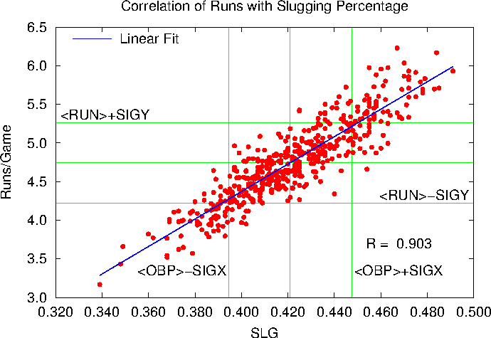
How about pure slugging:

Here R = 0.9026, where above R = 0.9031. OBS and SLG correlate equally well with Runs per game.

So what about everybody's favorite one-number way to evaluate a player?

Here R = 0.952. So our conclusion is that OPS is very well coordinated with Runs scored per game. Better than OBP or SLG, and far better than the batting average.

Now we could do all of this with fancy statistical packages, but for simple stuff like this we can do it all with gnuplot and see everything graphically.

Now that's the story for a very simple set of statistics. What about something like Runs Created? Is it really correlated with Runs per Game? Next time …

The Stalker Trilogy

As a teenager I loved the first two of these songs. But put back-to-back-to-back, there is a rather disturbing progression.

The Association Cherish (1966)

The Temptations Just My Imagination (Running Away With Me) (1971)

The Police Every Breath You Take (1983)

Insert Joel and Ethan Coen Reference Here

So in today's paper there's an Office Depot ad for a Brother HL 2240 Monochrome Laser Printer for $69.95. We really need a BW printer, and Laser is obviously the way to go to keep the price per page down. The thing got decent user reviews on Amazon, as long as you remember:

• It's Cheap.
• It's USB.
• You have to replace the drum at 14,000 pages (like we'll get to that any time soon).
• The initial cartridge only lasts for 700 pages (though you can apparently fool the printer into printing more)
• It's cheap.

So I went out and bought the thing — the closest thing to an impulse electronics buy since I got that $20 Canon Printer/Scanner when I was at Duke. (The scanner still works, the paper feed mechanism for the printer is broken.)

I read all of the installation instructions, plugged the thing in, printed the test page, got the USB cable from the $20 printer and used it to connect the printer with Hal, and turned on the printer. Ubuntu's auto print installer came up, recognized the printer, and …

Wouldn't you know it, CUPS doesn't have a driver for the Brother HL2240. (Obviously I didn't do a lot of research.)

No problem, Brother provides proprietary drivers for the printer. (Forgive me, St. Richard.)

It's not a difficult process. Go to Brother site, and download the .deb packages for the HL-2240:
LPR Driver (hl2240lpr-2.1.0-1.i386.deb) and
CUPS wrapper drive (cupswrapperHL2240-2.0.4-2.i386.deb).

Install both drivers, in order:

sudo dpkg -i --force-all hl2240lpr-2.1.0-1.i386.deb
sudo dpkg -i --force-all cupswrapperHL2240-2.0.4-2.i386.deb

At some point during this you'll get a message that the Brother printer has been found, and if you click on System Settings (under your name in the upper right of your screen), followed by Printers, and then Brother HL2240, you'll be able to print out the test page.

It works fine. Except …

I also want to be able to access the printer from Harlie, the machine upstairs. I previously alluded to doing this before (see rants, uh, points, 35 and 36), but that was with native CUPS drivers. I'll provide a bit more detail this time. Remember that the printer is installed on Hal, and we want Harlie to be able to use it.

So on Hal:

• Open up a browser and go to http://localhost:631/.
• Click on the Administration tab.
• Under Server on the right, click the box that says Share printers connected to this system, and then click Change Settings.

Go upstairs to Harlie:

• Install those same Brother Printer Drivers. You'll get some message about a printer being found. Ignore it.
• Open up a browser and go to http://localhost:631/.
• Click on Administration and Add Printer.
• You should see a box which says something like
  Brother HL2240 BW Laser @ harlie (Brother HL2240 series)
  Click its radio button and then click Continue.
• Fill in the information you want to use to identify the printer. Click Share this printer if you want others to be able to use it from Harlie. Again click Continue.
• Now for the trick. The next screen will ask you for the location of the CUPS driver. It won't be in the list, since it's proprietary, but after a bit of searching, I found it. Where it says Or Provide PPD File: click Choose File, and search until you find the file
  /usr/share/ppd/HL2240.ppd
  Choose this, then Add Printer.
• If the Force is With You, your printer will now be installed.

Note that you can use CUPS to change the behavior of your printer. For example, if you go to Administration, click on Manage Printers, and click the name of your printer, you'll see a page that has two pull-down boxes, one labeled Maintenance and the other Administration. Click on the Admin box and you'll see a bunch of things you can do. In particular, under Set Default Options you can choose your paper size, print resolution, ink toner usage, etc.

Finding Files Born After a Given Date

A few weeks ago Friend TK came up with a question:

RC, how can I find all of the pictures I put on my computer since Christmas without seeing all of the pictures in the .cache directories and other junk places?

An interesting question, indeed. We want to search for files that are newer than a certain target date, and they'll probably have extensions like .jpg or .png, though there will be the occasional file with an extension .jpeg or even .JPEG. It obviously requires some form of the Unix find command, but it's not exactly obvious what that would be. TK and I hunted around on the web a bit and finally came up with this:

touch -d 20111225 tokenfile
find . -type f \( -iname "*jpg" -o -iname "*jpeg" \) -anewer tokenfile  -print | egrep -v ".cache/|.thumbnails|.kde/"

which creates a marker, tokenfile, which looks to have been born last Christmas Day, and finds all files newer than that and ending in jpg or (the -o) jpeg without regard to case (that's the -iname). We then pipe the file through egrep, striping off (-v) files who have names matching directories we don't want to see (the | is the grep equivalent of find's -o.

This is not entirely elegant. I was pretty sure I could make this into a purely find one-liner, leaving no trace behind (such as that tokenfile we created up there. To do this I knew I'd have to delve deeper into findology than I had in my 30 or so years of Unix use. If found some of the clues at Linux.ie's finder-keepers page, and other hints elsewhere. Eventually this let me put together this one-line script:

find . -type d \( -iname .\[a-z\]\* -o -iname work \) -prune -o -newermt 2011225 \( -iname "*j*g" -o -iname "*png" \) -print

Let's look at this in some detail, since it contains some things that I hadn't known:

• find, of course, is the Unix/Linux command for looking through your file system.
• . is the current directory. Find uses it as the starting directory. find will look at every file in this directory, its sub-directories, and all their children and grandchildren, to the umpteenth generation. If you only wanted to search where you thought pictures might be, you could instead write
  find $HOME/Pictures
• -type d says that the next set of files will describe directories, rather than files (which would be -type f).
• The \( and \) delineate what will be a list of file descriptors. The backslashes make sure that the parenthesis are passed to find, and not gobbled up by the shell. Sometimes you can use quotations marks within find, instead of parenthesis, but this isn't one of those times.
• Now for the heart of the matter: -iname .\[a-z\]\* tells find to look for directory names that start with a . followed by a letter ([a-z]), and then by anything else (*). Again the backslashes are there to make sure the next characters are passed to the find command. Note that this gets rid of every hidden directory in you file tree.
• As before, -o is the or command. The -iname work command identifies my work directory, which may have pictures in it but nothing I'm interested in at the present time. You can add further -o -iname commands as needed.
• -prune tells find to look at every file except those in the directories just named. This serves the purpose of the egrep -v command in our initial attempt.
• You know, I'm not sure why the -o follows -prune. You'd think it would be some kind of and command, but just dropping it doesn't work.
• -newermt 20111225 is one of the newer options in find. This one says to look at all files modified (m) after a certain time (t). The time here is a date, written in the format yyyymmdd, in this case last Christmas. If we wanted files written after noon on Christmas, we'd use -newermt "20111225 1200".
• Again we have a list of -inames, delineated by backslash-parenthesis. These are file names you want to look for. Note that j*g catches all files ending in jpg, jpeg, JPG, or JPEG. It also catches files in .jynormouslyinteresting, but you can't have everything.
• Finally, -print lists all the files. You can actually drop this, as find takes -print as its default action.

And that's it. OK, not quite. What TK wanted was to copy all of the files he found to a new directory, we'll call it recent, so he could examine them in detail. To do that we use the -exec option of find:

find . -type d \( -iname .\[a-z\]\* -o -name work -o -name recent \) -prune -o -newermt 20111225 \( -iname "*j*g" -o -iname "*png" \) -exec cp -p {} ~/recent ';'

• Note that we've added the recent directory to our list of avoided directories. Otherwise find will search recent, and give errors.
• -exec tells find to execute the following file command.
• cp -r is the usual copy command, with -r saying to preserve the original timestamps on the copied files. If you wanted to save space, and weren't going to modify the pictures, you could link with either ln or ln -s instead.
• {} is where find places its output. That is, if there is a file Pictures/cutekids.jpg, find issues the command
  cp -r Pictures/cutekids.jpg recent
• ; tells find that we're done.

A Linux Preview Script

Mac OS X comes with a program called Preview, which displays PDF files as well as images (PNG, GIF, Bitmap, etc.). Linux doesn't have anything quite like it. OK, if you use the Gnome desktop there's something called Document Viewer, usually linked to evince, which reads Postscript, PDF, Djvu, DVI, etc. In fact, it displays Documents better than Preview does.

Unfortunately, evince doesn't display images. For that we have programs like Eye of Gnome, qiv (my favorite), and for image manipulation ImageMagick or the GIMP.

And then there are plain old ASCII files, such as you'd use for source code or LaTeX. For that we could use The One True Editor, or gedit, or some other sort of pop-up display window that lists the contents of a file.

What we want, then, is a program, preferably a command line script, which is given a file name, determines what the file is, and then opens the file using the appropriate viewer/editor. How do we do that, pray tell?

Enter the file command, inherited from Unix. file is pretty useful. For example, suppose I have a JPEG file, but for some reason it has been named x1, without the extension. file figures it out pretty fast:

$ file x1
x1: JPEG image data, JFIF standard 1.02

And it will work on most standard Linux file types.

Given this, it's fairly easy to construct a script which takes a look at one or more files, determines the file type, and picks out the approriate file viewer. My script is below. I've called it gnuview. You invoke it from the command line:

$ gnuview file1.txt file2.png file3.dvi file4.bmp

and all of these files pop up on your screen, each launched using the appropriate program.

A few notes:

• The list of file types is not by any means complete, though I think I hit most of the major ones. If the script doesn't know how to handle a specific file type, it prints out a message on standard error. It's fairly obvious how to add different file types.
• I dumped my favorite programs (qiv and emacs), in favor of programs that are installed by default with most Linux distributions (eye of gnome, gedit). (qiv doesn't read bitmap files, anyway.) Feel free to change the defaults to your favorite.
• Error messages? We don't need no stinkin' error messages!
• Finally, the cascading tree structure of if statements is just annoying. This should probably be rewritten using some kind of case construction, but I didn't bother to figure it out.

No warranty for any of this, of course, and not even a license except for the Creative Commons Disclaimer down at the bottom of this web page. If you come up with a version of this code, put it in the comments or put a link to it there.

#! /bin/bash

# This is an attempt to mimic the behavior of Apple's OS X Preview
#  program.  We determine the type of the file and then use the
#  appropriate command to open it.

# Some defaults.  Change as you see fit:

# ASCII files.  Note that gedit must be invoked in standalone mode

GNTXT="/usr/bin/gedit -s"

# Picture viewer (eog reads more files than qiv, so we'll use that)

GNPIC=/usr/bin/eog

# Postscript/PDF/DjVu/DVI viewer:

GNPDF=/usr/bin/evince

# Read the command line, and scroll through each file type:

for thisfile
do

#   If the string says ASCII anywhere, do this, which should get
#     LaTeX source, source code, etc.

    file $thisfile | grep 'ASCII' 2>&1 > /dev/null
    if [ $? -eq 0 ]
    then

        $GNTXT $thisfile &

    else

#   Maybe it's a document (Postscript/PDF/DjVu/DVI):
#   (I wan't sure about the "or" construct, see the first comment in
#   http://www.cyberciti.biz/faq/searching-multiple-words-string-using-grep/)
        file $thisfile | grep 'document\|DVI' 2>&1 > /dev/null
        if [ $? -eq 0 ]
        then
            $GNPDF $thisfile &
        else

#   Or maybe it's an image
            file $thisfile | grep 'image\|bitmap' 2>&1 > /dev/null
            if [ $? -eq 0 ]
            then
                $GNPIC $thisfile &
            else

#               And if we haven't figured out the type yet,
#                leave a nice note:
                FTYPE=`file $thisfile | awk '{print $2}'`
                echo Cannot handle file $thisfile, type $FTYPE  > /dev/stderr
            fi
        fi
    fi

done

Hoping we never have to play Illinois.

Poster format courtesy of Motivator

Cleanup Time

I promised my wife that I'd spend most of this long weekend cleaning up the office. It's been a while since I got my desk cleaned off, not to mention the various piles of clutter hiding in various corners.

I'm about halfway finished. It's been interesting. So far I've found:

• A $200 Series I savings bond — from 2007. I think I'll keep that.
• Family Circus Our House, a CD with what seems to be a game that lets you make like Billy and explore the house and neighborhood. For MS-DOS, at least it tells you to type D:\setup.exe on the command line. Takes up 3 MB of space. Never played. I think I'll send it to Stephan Pastis.
• Manual for lawnmower purchased in 1996 and broken down by 1998.
• About 50 blank 3-1/2 inch floppy disks. You want 'em, come get 'em.
• A Gateway 2000 System CD, from my very first Intel computer — I started with an Apple //e (see below).
• A copy of Microsoft Flight Simulator. Keeping that, I think it still plays either with Wine or Windows under VirtualBox.
• A wide variety of cheap CD encyclopedias, all dating from before Wikipedia, and even before that great and wonderful time when the Encyclopedia Britannica was online in its entirety, and free.
• The very first CD version of Halliday and Resnick's Fundamentals of Physics. I got it in return for writing a review for GEnie. It should be in my collection of reviews, but darned if I can find it.
• Zip Disks. Sans drive, of course.
• A Sherlock Holmes mystery game, complete with a large sheet of paper giving various clues. Also apparently for DOS, and also never played. Why did I buy this stuff?
• 5-1/4 inch (Yes) floppies for Appleworks, the Apple ][ spreadsheet/word processing/database software. There are even a pair of 3-1/2 inch floppies with it, and it runs on ProDOS, so apparently I bought it quite late in the game. I'm pretty sure my library database, circa 1990, is on another floppy somewhere.
• Along with that, big floppies of Sargon II, the great chess program. I actually played this one. Not well.
• And finally, a classic: 3-12 inch floppies for Borland Sidekick, the first great TSR (terminate and stay resident) program, and a great little calculator/calendar/whatever. You could pop it up, type in a note, go back to playing whatever text-based game you were playing, stop, type in another note, etc., all without going back the command line prompt. A great program for its time.

There are more nooks and crannies around here, if I find anything interesting tomorrow I'll let you know.

Public Service Announcement

Resize a Lot of Pictures

The church web site I run has a box the displays random pictures from our photo album. The formatting of the page is easiest if these pictures are no wider than 530 pixels and no higher than 340 pixels. Of course most pictures are taken with a camera these days are a couple of thousand pixels wide, so each picture needs to be resized. You can do that by hand, of course, but I found it easiest to write a script. If you're running Linux, this uses the ImageMagick package, particularly the identify and convert programs. On a Mac, it uses sips, which has been available at least since 10.3. I suppose it could be modified for Windows or run under Cygwin, but I don't use Windows enough to make it worth my time.

Save the file as websize, make it executable, and save it to a directory in your path. Then run it with the command

websize [list of image files]

This will take a file named, say, picture1.jpg, and create a new file named picture1_web.jpg that fits into the box defined by MAXWIDTH and MAXHEIGHT. If the picture already fits into the box it will duplicate the file.

#! /bin/bash

# Resizes a picture or pictures to make sure it fits into the UPB
# frontpage box of MAXWIDTH pixels wide by MAXHEIGHT pixels tall,
# keeping the same format (PNG, JPEG, BMP, etc.)

# usage

# websize [pictures]

# If a picture is named "picturename.ext", the shrunken picture
#  will be named "picturename_web.ext".

# If a picture already fits into the website, it will simply be
#  copied with its new name.  This makes it easier to find the
#  pictures that should be posted on the web.

# Define the maximum dimensions of the picture

let MAXWIDTH=530
let MAXHEIGHT=340

# For Linux machines we need "convert" from the ImageMagick package.
#  We'll assume it's in the standard location:

# For Macs the standard program is sips, at least since 10.3

if [ -f /usr/bin/sips ]
then
    OS="Mac"
elif [ -f /usr/bin/convert ]
then
    OS="Linux"
else
    echo "Cannot find a program to do the file conversion"
    exit 1
fi

for PICTURE
do

if [ "$OS" = "Linux" ]
then

#   identify is also part of the ImageMagick package

    let WIDTH=`identify $PICTURE | sed "s/x/ /" | awk '{print $3}'`
else
    let WIDTH=`sips -g pixelWidth $PICTURE | tail -1 | awk '{print $2}'`
fi

# Need new picture name:

HEADER=${PICTURE%.*}
EXT=${PICTURE##*.}
NEWPICT=${HEADER}_web.$EXT

echo Converting $PICTURE to $NEWPICT

# Is the picture too wide?

if (( $WIDTH > $MAXWIDTH ))
then
    if [ "$OS" = "Linux" ]
    then
 convert -resize ${MAXWIDTH}x $PICTURE $NEWPICT
    else
 sips --resampleWidth $MAXWIDTH $PICTURE --out $NEWPICT
    fi
else
    cp $PICTURE $NEWPICT
fi

# Note that the new picture may still be too large:

if [ "$OS" = "Linux" ]
then
    let HEIGHT=`identify $NEWPICT | sed "s/x/ /" | awk '{print $4}'`
else
    let HEIGHT=`sips -g pixelHeight $NEWPICT | tail -1 | awk '{print $2}'`
fi

if (( $HEIGHT > $MAXHEIGHT ))
then
#   echo Resizing height of $PICTURE

    if [ "$OS" = "Linux" ]
    then
 convert -resize x$MAXHEIGHT $NEWPICT 1_${NEWPICT}
    else
 sips --resampleHeight $MAXHEIGHT $NEWPICT --out 1_$NEWPICT
    fi

    mv 1_${NEWPICT} $NEWPICT

fi

done

The obvious modification is to allow MAXWIDTH and MAXHEIGHT to be read from the command line, maybe using -w and -h flags. That's for another day.

Joining a Group

In an effort to make Ubuntu less scary to users (i.e., more Mac/Windows like), Ubuntu 11.10 removed some graphical system administration utilities that were previously available. One of those was a called Users and Groups, which let you see groups and make changes to group memberships.

The new Ubuntu would rather you just forget groups, so it includes no graphical tools for handling them. Fortunately it's still Linux, so you can fix it up yourself. Liberian Geek has details, but the first hint (using groupmod) didn't work for me, so here's my modified version. In this example, I want to add myself to the group vboxusers, which should allow me to get USB access for my Virtualbox installation. More on that some other time. For now, return with us to those thrilling days of yesteryear, before the GUI:

1. Look at the file /etc/group. Specifically, we want to see who belongs to the group vboxusers:

   $ grep vboxusers /etc/group
   vboxusers:x:125:
   

   Nobody, as we expected.
2. Now to follow the Geek and add myself:

   sudo usermod -a -G vboxusers rchawk
   

3. Finally, confirm the addition

   $ grep vboxusers /etc/group
   vboxusers:x:125:rcjhawk
   

You'll need to log out and log back in before the system will recognize the new group setting.